Welcome to my personal webpage. | home
Driver Amplifier and Low Pass Filter | Butterworth Low-Pass Filters and Applications of Spectrum Analyzer | BJT Amplifiers | MOSFET CS Amplifiers with Active Load | Common Emitter Circuit | ACCELEOMETER SENSOR | Diode Waveform Shaping
Butterworth Low-Pass Filters and Applications of Spectrum Analyzer
EE 403W
Spring 2003
Nima Moshtagh
Introduction
Filters are widely used in communication and signal-processing systems. There are different types of filters such as low-pass, high-pass and band-pass filters. These filters are usually made of resistors, capacitors and operational amplifiers (op-amps). In this lab we consider only 2nd order filters. The transfer function of a 2nd order filter has 2 poles and looks like
 (1)
(1) where ù is the pole frequency and Q is the pole. The filter that its transfer function most closely approximates the asymptotic lines of a Bode diagram while having a monotonic slope is called Butterworth Filter.
The goal in this lab is to design a Butterworth low-pass filter. We will test the circuit by a rectangular wave signal which is a square wave with 30% duty cycle.
B1 - Asymmetrical Square Wave
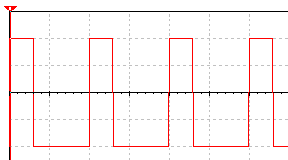
Before designing the low-pass filter, we analyze a periodic asymmetrical square wave using a Spectrum Analyzer HP3561A. An asymmetrical square wave is shown in figure 1. The duty cycle of the signal is 30%, meaning that signal is high for 30% of one period and it is low for the next 70% of a period.

Figure 1) 30% duty cycle square wave
When we apply this signal to the spectrum analyzer, it shows the components of this signal in the frequency domain. Attachment A shows what we saw on the display of the Spectrum Analyzer. Each component represents the magnitude of the corresponding term in the Fourier series of the signal. Fourier series representation of a signal has the general form of
where a0 is the dc component of the signal. An and Bn, for a signal with the duty cycle of D, are given by
where A is the amplitude of the signal. Refer to appendix B for derivation of these expressions. The magnitude of each term can be calculated by using the Pythagorean Theorem and will be simplified to
First we analyzed a 50% duty cycle square wave with the frequency of 1 kHz and 10 volts peak-to-peak. When D = 0.5, for even values of n (n = 2,4,6,
), the theoretical values of the even harmonics must be zero:
The experimental values of the even harmonics were very small but non-zero values. The measurements were given in dBV on the display and we needed to convert them back to Volts. We learned that the Spectrum Analyzer measures the rms values of signals. Thus, we needed to include a factor of  for amplitude calculations. The conversion is as follows:
We measured the magnitude of even harmonics to be -45.87 dB, or 7.19 mV which is still very small compared to the amplitude of the signal. A possible explanation could be that the original rectangular signal is not an ideal signal and it contains some noise.
Then we applied a 10 volt peak-to-peak, 1kHz, 30% duty cycle square signal to the analyzer and table 1 compares the theoretical and experimental values of the fundamental, 2nd and 3rd harmonics of the signal (See attachment A). Theoretical and experimental values match up with less than 0.2% error.
Harmonics
|
Theoretical (V)
|
Experimental (V)
|
Experimental (dB)
|
á 0
|
-2
|
3.0
|
9.5
|
1
|
5.15
|
5.14
|
11.21
|
2
|
3.02
|
3.02
|
6.6
|
3
|
0.655
|
0.656
|
-6.67
|
Table 1) Comparison of theoretical and experimental values of fundamental, 2nd and 3rd harmonics of 30% duty cycle square wave.
The only obvious difference between theoretical and experimental values was for the dc component of the signal. The dc component is calculated to be -2 volts but spectrum analyzer measures it to be 3.0 volts. It appears that since the dc component is less than zero, the analyzer adds the value of the peak voltage (+5V) to the negative voltage (-2V) so that a positive voltage of +3V can be displayed.
B2 - Butterworth Low-Pass Filter
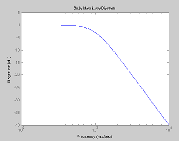
Now we are going to design a low-pass filter (LPF) by using active elements such as op-amps to avoid using conductors. The frequency response of an ideal low-pass filter is shown in figure 2. A LPF is supposed to filter out higher frequencies and pass only frequencies that fall in its bandwidth (below the cut-off frequency).

Figure2) Magnitude Response of an Ideal Low-Pass Filter.
The design specification is asking for a second order Butterworth low-pass filter with a single op-amp, a cutoff frequency of 1 kHz and unity DC gain. Therefore, in equation (1) ù0 = 2p*1000 Hz = 6283 Hz. The value of Q is determined to be Q = 0.707 for second order Butterworth filters. For Q > 0.707 resonance will happen at ù0 which is not desirable.
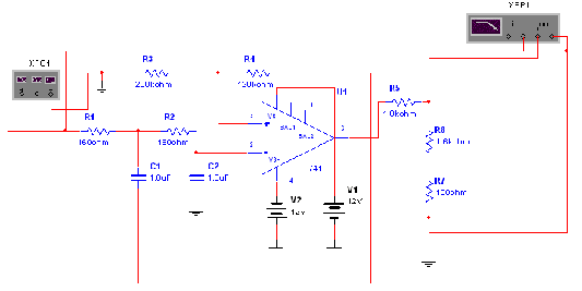
A single op-amp, second order active RC Filter that was built by our team is shown in figure 3.

Figure 3) Low-Pass Filter circuit Design
The DC gain of this filter was Gain = , therefore we had to design an attenuator to bring it down to 1. The design calculations are shown in the attachment C. But a summary is provided here.
R1 = R2 = 160W
C1 = C2 = 1mF
Ra = 120kW Rb = 203kW
Rx = 1kW Ry = 1.7kW
B3 - Measurement of Filter Transfer Function
We applied a pseudorandom signal, taken from the SOURCE OUTPUT jack of the spectrum analyzer, to our filter. This random signal contains different frequencies and is suitable for Spectrum measurements. A plot of the frequency response of the filter is provided in Attachment D. Unfortunately, the analyzer was not able to send the entire graph to the printer, and thus we have only half of the displayed frequency response. Table 2 compares the desired specifications and the achieved results.
desired
|
Achieved
|
|
Low-Frequency Gain
|
1
|
1.02
|
Break Frequency (Hz)
|
1000
|
1025
|
High Frequency Slope (dB)
|
-40
|
-30
|
Table2 - Comparison of the desired and Achieved specifications
Since the system is 2nd order, it has 2 poles on the left-half plane and each one contributes -20 (dB/decade) to the slope of the magnitude response. Therefore, the high frequency slope must be -40 (dB/decade). The proof is as follows: The magnitude of a low-pass filter is given by

where ùc is the cutoff frequency and n is the order of the filter. For ù >> ùc we have

for two frequencies ù1,ù2 >> ùc and ù2 = 10*ù1 we get
therefore 
And we can see that if the system is second order (n = 2), the magnitude difference for two frequencies that are 1 decade apart is -40 dB. The approximate measured slope was -30 (dB/decade) which is significantly smaller than what we expected. A possible reason could be the error in measurement, because the transfer function gets very noisy at high frequencies and that makes the measurements unreliable.
B4 - Spectrum of the Filtered Asymmetrical Square Wave
Now that both input signal and filter are ready, we can apply the input to the system and witness that our filter attenuates high frequencies much more than lower ones. Plots of the attachment E show both input and output signals in the frequency domain. A comparison between the magnitude of different harmonics in input and output signals is provided in Table 3.
Harmonics
|
Input (volts)
|
Output (Volts)
|
Vout / Vin
|
0
|
4.22
|
3.98
|
0.944
|
1
|
5.18
|
2.76
|
0.534
|
2
|
3.02
|
0.12
|
0.041
|
3
|
0.66
|
0.095
|
0.145
|
4
|
1.00
|
0.20
|
0.200
|
5
|
1.34
|
0.25
|
0.188
|
6
|
0.63
|
0.11
|
0.178
|
Table 3 - Magnitude Comparison of Different Harmonics in the Input and Output Signals
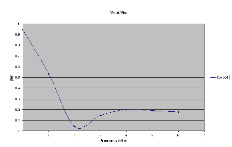
Figure 4 shows the experimental frequency response of the filter. It demonstrates how the LPF attenuates different frequencies. As one can see small frequencies are not attenuated at all, while components with larger frequencies are almost entirely removed from the signal.

Figure 4) The experimental Frequency response of the designed low-pass filter.
B5 - Time Domain Plots of the Input and Output
A square wave has sharp points and those correspond to high frequencies in the Fourier series. When we pass a square wave through a lop-pass filter, all the high frequencies will be removed. In other words, sharp points in the input signal would disappear in the output signal. Attachment F compares the input and output signals in the time domain. As it appears, the output has lost the sharp transitions and it looks more like a sinusoid.
Conclusions and Discussions
Butterworth filters approximate the asymptote lines of the Bode plot of a filter. In the transition interval of the filter, the magnitude falls monotonically with -20N (dB/decade) in which N is the order of the Butterworth filter. To be able to analyze what happens to a signal when it goes through the filter, we should consider the Fourier series of the signal. In our experiment we used a 30% duty cycle square wave. The Fourier series of a square wave has high frequency and low frequency components. Our experiments showed that a low-pass filter (LPF) will block all the frequencies that are much higher than the break-frequency. Since our filter had a unity DC gain the dc components of the input signal was not attenuated at all.
To build a LPF we designed an active filter by using resistors and capacitors and one opamp. Since the gain of the filter was more than unity, we had to put an attenuator at the output. The attenuator was a simple voltage divider. We observed that the output signal of the filter would not have fast transitions of the input (sharp corners were removed). Because sharp corners correspond to high frequencies, our low-pass filter removed them from the input.